[WITH CODE] Models: Signal independence

What is the best way to turn signals into alpha? A quant's guide to avoiding beta gridlock

---

Table of content:

1. Introduction.

2. What are raw signals, anyway?

3. Transforming raw signals into alpha.

4. Why does independence matters?

5. What’s the best way to pick the right signals?

---

Introduction

If you’ve spent any time in the quant world, you know that financial markets are like a never-ending, crowded city at rush hour. Every asset is an intersection, and every trading signal is a traffic light—some blinking perfectly in sync, others flickering unpredictably. As quants—or as I like to call us, the urban planners of finance—, our job is to turn these raw signals into actionable trading ideas—alpha—without getting stuck in a beta-induced gridlock.

Now, before you get too excited, let’s make one thing clear: more isn’t always better. Just as adding too many traffic signals in a city might just confuse drivers, compounding multiple trading rules doesn’t automatically give you extra alpha. Sometimes you get additional risk exposure—beta—that makes you wonder if you’re driving a convertible on a rainy day.

The other day in an article, I mentioned this:

Adding rules reduces your chances of winning, even if each rule is slightly good. Every added rule introduces a new chance to fail. Complexity isn’t just confusing—it’s mathematically self-sabotaging.

Take a look, you’re going to like it. Now, I think some things should be clarified regarding that phrase, and that’s what we’re going to cover today—because it depends on the system you use, the type of signal it picks up, how the exit occurs, and many other factors.

So, imagine walking through a city where every street corner has a sign. Some signs give useful directions, while others are outdated or simply wrong. Each asset comes with its own raw signal—be it momentum, volatility, or earnings. These signals, in their original form, are like those confusing street signs: they might point you in the right direction, but more often than not, they need some fine-tuning.

What are raw signals, anyway?

Let’s denote the raw signal for asset i by sis_isi​. With N assets in your portfolio, you have a list of signals s₁,s₂,…,s_N​ that might be all over the place—just like the eclectic mix of taxi drivers in a big city. Our first job is to standardize these signals so that we can compare them fairly. Enter the Z-score.

The Z-score for asset iii is given by:

\(z_i = \frac{s_i - \mu_s}{\sigma_s}, \)

Where:

• μ_s​ is the mean of all signals, and

• σ_s is the standard deviation.

Think of it as adjusting every street sign in the city so they’re all in the same language—helpful, right?

Relying on just one signal is like trusting a single traffic light to control a chaotic intersection. Sure, if that one light is working perfectly, you might cruise through the city. But what if it malfunctions? That’s why some quants like to combine multiple signals.

But, the big question remains: When you mix a few signals together, are you getting a superior, well-coordinated system—more alpha—, or are you just compounding your exposure to market risk—more beta—?

Transforming raw signals into alpha

Before we can talk about combining rules, we need to know how to transform our raw signals into something that matters—alpha. In our trading world, alpha is that elusive extra return, the secret sauce that separates winners from losers. Think of it as upgrading from a beat-up sedan to a sleek sports car—with air conditioning, of course.

A widely used transformation in our field—yes, even us senior quants have our old-school formulas—is:

\(\alpha_i = \sigma_i \cdot IC_i \cdot z_i. \)

Let’s break that down:

• σ_i​: This is the residual volatility of asset i—in other words, the “spice” that adds unpredictability to our returns. Imagine a street that sometimes has potholes for no apparent reason.

• IC_i​: The Information Coefficient, or IC, measures how good your signal is at predicting future returns. An IC of 0 is as useful as a broken GPS, while an IC of 0.1 might get you to your destination 53% of the time—which is better than random guessing, but still makes you want to double-check the route.

• z_i: That trusty Z-score which normalizes our raw signal.

Put these together, and you have a neat little formula that transforms messy, raw data into something you can actually trade on.

A quick example, let’s say we have a set of momentum signals for 10 assets:

import numpy as np

# Raw momentum signals for 10 assets—think of these as our city’s street ratings
momentum = np.array([12, 15, 10, 8, 20, 5, 18, 9, 14, 7])

# Calculate mean and standard deviation
mean_mom = np.mean(momentum)
std_mom = np.std(momentum)

# Compute Z-scores: adjusting all our signals to a common standard
z_scores = (momentum - mean_mom) / std_mom
print("Z-scores:", z_scores)

# Define our constants—residual volatility (like the bumps in the road) and IC (signal quality)
volatility = 0.2
IC = 0.1

# Compute alpha for each asset: our version of transforming chaos into potential profit
alpha = volatility * IC * z_scores
print("Alpha values:", alpha)

# Output:
# Z-scores: [ 0.04307305  0.68916879 -0.38765744 -0.81838794  1.76599502 -1.46448367, 1.33526453 -0.60302269  0.47380354 -1.03375318]
# Alpha values: [ 0.00086146  0.01378338 -0.00775315 -0.01636776  0.0353199  -0.02928967, 0.02670529 -0.01206045  0.00947607 -0.02067506]

We compute the mean and standard deviation of the momentum signals—our basic road conditions. Z-scores standardize these signals—as if every street sign were being replaced with a modern LED display. Multiplying by volatility and IC gives us the final alpha values.

In simple terms, positive alphas suggest buying this asset, while negative ones indicate selling it before it dampens your returns.

Now that we’ve seen how to cook up a single alpha, let’s talk about mixing multiple signals together. Assume you have M different signals for each asset. For the j-th signal for asset i, we calculate:

\(\alpha_{ij} = \sigma_i \cdot IC_{ij} \cdot z_{ij}. \)

Then, if we want a compounded rule, we simply combine them using weights w_j:

\(\alpha_i^{\text{combined}} = \sum_{j=1}^{M} w_j \alpha_{ij}. \)

In practice, a lot of us start with equal weights. But remember, the secret sauce is in how independent these signals are from one another.

Why does independence matters?

Let’s say your signals are as independent as the various neighborhoods in a sprawling city. Then each one is capturing a different slice of the market action. In that case, combining them helps reduce noise—like smoother traffic flow with well-timed lights.

Mathematically, if the signals are uncorrelated, the combined variance is given by:

\(\sigma_{\text{combined}}^2 = \sum_{j=1}^{M} w_j^2 (\sigma_i \cdot IC_{ij})^2. \)

This diversification is akin to not putting all your eggs in one basket—or in our case, not relying on a single, temperamental traffic light.

On the flip side, if your signals are highly correlated—like every streetlight in a district turning red at once—then the benefits of compounding evaporate. Instead of a symphony of independent signals, you just have a chorus of redundant rules, and that’s when you end up with more beta than alpha.

In other words, you might be exposed to more market risk than you bargained for, like getting caught in a traffic jam when you thought you’d found a shortcut.

For uncorrelated signals, the combined information coefficient is approximately:

\(\text{IC}_{\text{combined}} = \sqrt{\sum_{j=1}^{M} w_j^2 \cdot IC_{ij}^2}. \)

If we assign equal weights (w_j=1/M), then this simplifies to:

\(\text{IC}_{\text{combined}} = \frac{1}{\sqrt{M}} \sqrt{\sum_{j=1}^{M} IC_{ij}^2}. \)

This result tells us that—even though adding signals improves our overall prediction—the marginal benefit shrinks as you pile on more signals. It’s like adding one extra taxi in a city already crawling with rides: it might help, but only up to a point.

Let’s now see how the quality of our signal impacts our Sharpe ratio—your task for today is to explore an alternative metric, ideally one that offers improved performance or insights. We can simulate this with this snippet:

import numpy as np
import matplotlib.pyplot as plt

def simulate_momentum_strategy(IC, n_days=252, n_stocks=200):
    """
    Simulate a momentum strategy for a given Information Coefficient (IC).
    Returns the annualized Sharpe ratio of a long-short top/bottom 20% approach.
    """
    # Daily returns storage
    daily_returns = []

    for _ in range(n_days):
        # 1) Generate random alpha signals for each stock (standard normal)
        alpha_signals = np.random.randn(n_stocks)

        # 2) Generate next-day stock returns correlated with alpha_signals by IC
        #    r = IC * alpha + sqrt(1 - IC^2) * noise
        noise = np.random.randn(n_stocks)
        stock_returns = IC * alpha_signals + np.sqrt(1 - IC**2) * noise

        # 3) Rank stocks by alpha, long top 20%, short bottom 20%
        #    We'll approximate the daily strategy return as the average of
        #    returns in the long bucket minus the average of returns in the short bucket.
        cutoff = int(0.2 * n_stocks)
        # Sort stocks by alpha descending
        sort_idx = np.argsort(alpha_signals)[::-1]

        top_returns = stock_returns[sort_idx[:cutoff]].mean()
        bottom_returns = stock_returns[sort_idx[-cutoff:]].mean()

        strategy_return = top_returns - bottom_returns
        daily_returns.append(strategy_return)

    # 4) Convert daily returns into an annualized Sharpe ratio
    #    (simple approximation: sqrt(252) * mean(daily_ret) / std(daily_ret))
    daily_returns = np.array(daily_returns)
    avg_daily_ret = np.mean(daily_returns)
    vol_daily_ret = np.std(daily_returns)

    if vol_daily_ret == 0:
        return 0.0

    sharpe_daily = avg_daily_ret / vol_daily_ret
    sharpe_annualized = sharpe_daily * np.sqrt(252)
    return sharpe_annualized


# Sweep a range of IC values from 0 to 0.2
IC_values = np.linspace(0, 0.2, 11)

# Run multiple simulations per IC to smooth out randomness
n_sims = 10
avg_sharpes = []

for ic in IC_values:
    sharpe_across_sims = [
        simulate_momentum_strategy(ic) for _ in range(n_sims)
    ]
    avg_sharpes.append(np.mean(sharpe_across_sims))

# Plot the relationship between IC and strategy performance (Sharpe ratio)
plt.figure(figsize=(8, 5))
plt.plot(IC_values, avg_sharpes, marker='o', label='Average Sharpe Ratio')
plt.xlabel('Information Coefficient (IC)')
plt.ylabel('Annualized Sharpe Ratio')
plt.title('Momentum Trading Alpha Performance vs. IC')
plt.grid(True)
plt.legend()
plt.show()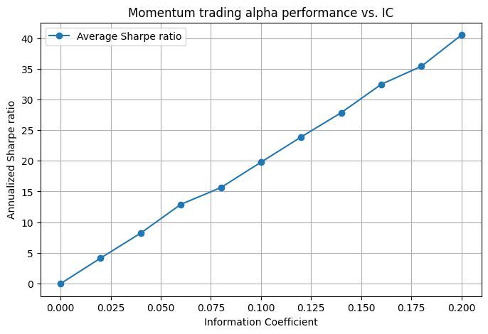

Remember, even with an IC of 0.1, our “accuracy”—I hate this word—is only marginally better than flipping a coin. So if your trading strategy were a carnival game, you’d still be on the side of fun rather than profitable.